Definition
When approximating a discrete distribution such as the Binomial or Poisson with a continuous distribution such as the Normal, a problem arises because discrete probabilities apply to integer values whereas continuous probabilities apply to intervals.
For instance, the binomial probability P(X=7) corresponds to P(6.5<X<7.5) under the normal distribution. Similarly, P(X≤7) becomes P(X<7.5) and P(X≥7) becomes P(X>6.5). Using the continuity correction (also called Yates’ continuity correction) allows us to fill in the ‘gaps’, giving a much closer approximation than would be otherwise obtained.
Examples

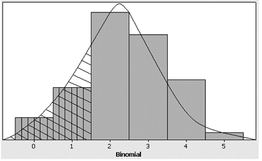
Consider the histogram of the distribution of X: Number of heads in 5 tosses of an unbiased coin. This is a binomial variable with parameters n=5 and p=0.5 (assuming heads and tails are equally likely). To find the probability of getting 1 or fewer heads, P(X≤1), we would add the frequencies corresponding to the values 0 and 1. This area is represented by the vertical lines through the first two bars, for 0 and 1.
However, the corresponding normal probability is represented by the area under the normal approximation curve covered by the diagonal lines. Obviously, the two areas are not exactly equal. In fact, the area under the continuous curve corresponds to the probability P(X<1.5). Thus, we add the continuity correction factor 0.5 to 1 to find the area less than or equal to 1.
Application
For the calculation of the Z test statistic in the Z-test for a single population mean, the continuity correction adds 0.5 to the numerator in the ‘less-than’ case and subtract 0.5 from the numerator in the ‘greater-than’ case.
External Links
A tutorial on the normal approximation to the binomial distribution: - http://facstaff.bloomu.edu/wblee/norapp.htm
